Example Application: Defect Detection of Workpieces in a Casting Manufacturing Process.

In this guide you’ll rapidly build a binary classifier to detect defects in a manufacturing process. Each workpiece is created using a casting manufacturing process, in which molten metal is poured into a mold.
You have been tasked with building a solution to satisfy the following user story:
As a plant manager,
I want to automatically detect defects in my workpieces,
so that I can deploy it alongside my existing manual QC process to reduce my plant's defect rate.
Your first task is to acquire data. Normally, you’d have to get up from your desk and start snapping photos with your phone, or install a camera over an assembly line and feed it to a server. For the purposes of this example, you’ll use an existing data set.
Acquiring Data
Go to kaggle.com and register an account. Follow these instructions to acquire a Kaggle API Token and save it to ~/.kaggle/kaggle.json. Install kaggle via pip, then download the dataset and unzip it, then get rid of the zip file. The data we care about it is in ./casting_512x512/casting_512x512. The two subdirectorys are def_front and ok_front, corresponding to defective and okay workpieces.
[2]:
!mkdir ~/.kaggle
!echo "{\"username\":\"YOUR_USERNAME\",\n\"key\":\"YOUR_KEY\"}" > ~/.kaggle/kaggle.json
[3]:
import sys
!{sys.executable} -m pip install --upgrade pip --quiet
!{sys.executable} -m pip install kaggle --quiet
!kaggle datasets download -d ravirajsinh45/real-life-industrial-dataset-of-casting-product
!ls *.zip
!unzip -q -o real-life-industrial-dataset-of-casting-product.zip
Exploratory Data Analysis
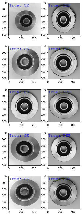
Next, it’s always important to perform EDA to search for any anomolies, errors, and to develop an intuition for your images and labels. As a bare minimum, visulize some OK and DEFective examples. The similarity of these images indicates that this dataset is low entropy, which would normally make hyperparameter tuning difficult. However, Masterful automatically handles hyperparameter tuning, so you will have no problems working with this low-entropy dataset.
[4]:
import matplotlib.pyplot as plt
import PIL, PIL.ImageDraw, PIL.ImageFont
import requests
from io import BytesIO

ok = [
    "./casting_512x512/casting_512x512/ok_front/cast_ok_0_1018.jpeg",
    "./casting_512x512/casting_512x512/ok_front/cast_ok_0_1021.jpeg",
    "./casting_512x512/casting_512x512/ok_front/cast_ok_0_1028.jpeg",
    "./casting_512x512/casting_512x512/ok_front/cast_ok_0_1074.jpeg",
    "./casting_512x512/casting_512x512/ok_front/cast_ok_0_1082.jpeg",
]

def_ = [
    "./casting_512x512/casting_512x512/def_front/cast_def_0_0.jpeg",
    "./casting_512x512/casting_512x512/def_front/cast_def_0_100.jpeg",
    "./casting_512x512/casting_512x512/def_front/cast_def_0_1015.jpeg",
    "./casting_512x512/casting_512x512/def_front/cast_def_0_102.jpeg",
    "./casting_512x512/casting_512x512/def_front/cast_def_0_1046.jpeg",
]

images = [ok, def_]
ROWS = 5
COLUMNS = len(images)

f, axarr = plt.subplots(ROWS, COLUMNS, figsize=(5,15))
curr_row = 0

for col, image_col, true in ((0, ok, 'OK'), (1, def_, 'DEF')):
    for row, image_row in enumerate(image_col):
        with PIL.Image.open(image_row) as image:
            drawing = PIL.ImageDraw.Draw(image)
            font = PIL.ImageFont.truetype('FreeMono.ttf', 65)
            drawing.text((10, 10), f'True: {true}', font=font, fill =(0, 0, 255))
            axarr[row, col].imshow(image)
Creating Labels
You’ll use the Masterful CLI Trainer to quickly train a model to state of the art performance. By using Masterful, you’ll avoid lots of the tedious parts of deep learning: setting up data processing pipelines, implementing architectures, and fiddling with hyperparameters. In fact, you may be able to avoid using experiment tracking tools entirely because Masterful automatically runs experiments to tune hyperparameters related to optimization, data augmentation, and regularization.
The Masterful label format is a simple CSV structure. Each row is a relative path, followed by an integer corresponding to a label. A second labelmap file maps those integers to short text descriptions.
Let’s generate and then examine a few lines of the csv.
[5]:
import os

OK_PATH = './casting_512x512/casting_512x512/ok_front/'
DEF_PATH = './casting_512x512/casting_512x512/def_front/'

ok = os.listdir(OK_PATH)
def_ = os.listdir(DEF_PATH)

print(f'num ok images: {len(ok)}. Using 10% for test: {len(ok)//10}')
print(f'num def images: {len(def_)}. Using 10% for test: {len(def_)//10}')

with open('test.csv', 'w') as f:
  for path in ok[:len(ok)//10]:
    f.write(OK_PATH + path + ',0\n')

  for path in def_[:len(def_)//10]:
    f.write(DEF_PATH + path + ',1\n')

with open('train.csv', 'w') as f:
  for path in ok[len(ok)//10:]:
    f.write(OK_PATH + path + ',0\n')

  for path in def_[len(def_)//10:]:
    f.write(DEF_PATH + path + ',1\n')
num ok images: 519. Using 10% for test: 51
num def images: 781. Using 10% for test: 78
[6]:
!head train.csv
./casting_512x512/casting_512x512/ok_front/cast_ok_0_6471.jpeg,0
./casting_512x512/casting_512x512/ok_front/cast_ok_0_5852.jpeg,0
./casting_512x512/casting_512x512/ok_front/cast_ok_0_4503.jpeg,0
./casting_512x512/casting_512x512/ok_front/cast_ok_0_1761.jpeg,0
./casting_512x512/casting_512x512/ok_front/cast_ok_0_9634.jpeg,0
./casting_512x512/casting_512x512/ok_front/cast_ok_0_7112.jpeg,0
./casting_512x512/casting_512x512/ok_front/cast_ok_0_1879.jpeg,0
./casting_512x512/casting_512x512/ok_front/cast_ok_0_6306.jpeg,0
./casting_512x512/casting_512x512/ok_front/cast_ok_0_3371.jpeg,0
./casting_512x512/casting_512x512/ok_front/cast_ok_0_8002.jpeg,0
Finally, create a simple label_map csv file, marking each image as OK or DEF (for defective).
[7]:
! echo -e "0, ok \n 1, def" > label_map.csv
YAML Config File for Masterful CLI Trainer
Now, you’ll setup the YAML config file. This config file is very sparse compared to YAML files you might have worked with in the past because the CLI Trainer is goal oriented. It is not simply wrapping a low level Python API in YAML - the CLI Trainer only needs to understand the goals for your model. Its internal automation handles the process of setting up data pipelines, training, regularization, evaluation, and saving the model.
The main decision you need to make in the config is which model architecture to train with. The decision on model architecture is a trade-off between inference speed and accuracy. The bigger the model, the slower and more expensive it will be to run in inference, but the more accurate it will be.
For a first training run, starting with the smallest possible model allows you to iterate more quickly. Then, once you have a trained model, you can experiment with larger models. One of the smallest available models is mobilenetv3_small.
dataset:
  root_path: .
  splits: [train, test]
  label_map: label_map

model:
  architecture: mobilenetv3_small
  num_classes: 1
  input_shape: [512,512,3]

training:
  task: binary_classification
  training_split: train

output:
  formats: [saved_model]
  path: ~/model_output

evaluation:
  split: test
[8]:
!touch config.yaml
!echo  "dataset:" > config.yaml
!echo  "  root_path: ." >> config.yaml
!echo  "  splits: [train, test]" >> config.yaml
!echo  "  label_map: label_map" >> config.yaml
!echo  "model:" >> config.yaml
!echo  "  architecture: mobilenetv3_small" >> config.yaml
!echo  "  num_classes: 1" >> config.yaml
!echo  "  input_shape: [512,512,3]" >> config.yaml
!echo  "training:" >> config.yaml
!echo  "  task: binary_classification" >> config.yaml
!echo  "  training_split: train" >> config.yaml
!echo  "output:" >> config.yaml
!echo  "  formats: [saved_model]" >> config.yaml
!echo  "  path: ~/model_output" >> config.yaml
!echo  "evaluation:" >> config.yaml
!echo  "  split: test" >> config.yaml

!cat config.yaml
dataset:
  root_path: .
  splits: [train, test]
  label_map: label_map
model:
  architecture: mobilenetv3_small
  num_classes: 1
  input_shape: [512,512,3]
training:
  task: binary_classification
  training_split: train
output:
  formats: [saved_model]
  path: ~/model_output
evaluation:
  split: test
Train
You are ready to train. Notice that you did NOT have to worry about:
Augmenting data with slow OpenCV / PIL CPU based transforms
Figuring out hyperparameters for regularization methods
Trying to implement state of the art augmentations
Tuning your learning rate and batch size and optimizer to make the most of your GPU
The training run will take about an hour on an Nvidia V100 GPU.
Once training is complete, the CLI will print out evaluation metrics and save the model to disk at model_ouput. You’ll have everything you need to see if the model meets your acceptance criteria.
[9]:
!{sys.executable} -m pip install -U masterful --quiet
!masterful-train --config=config.yaml
Loaded Masterful version 0.5.2. This software is distributed free of charge for
personal use. Register in the next 40 days to continue using Masterful.
Visit http://www.masterfulai.com/register for more details.

MASTERFUL [13:27:57]: Training with configuration 'config.yaml':
----------  -------------------------------------
dataset     root_path  .
            splits     ['train', 'test']
            label_map  label_map
model       architecture  mobilenetv3_small
            num_classes   1
            input_shape   [512, 512, 3]
training    task            binary_classification
            training_split  train
output      formats  ['saved_model']
            path     ~/model_output
evaluation  split  test
----------  -------------------------------------
MASTERFUL [13:27:58]: Building model 'mobilenetv3_small'...
MASTERFUL [13:27:59]: Using model mobilenetv3_small with:
MASTERFUL [13:27:59]:     1530993 total parameters
MASTERFUL [13:27:59]:     1518881 trainable parameters
MASTERFUL [13:27:59]:     12112 untrainable parameters
MASTERFUL [13:27:59]: Dataset Summary:
MASTERFUL [13:27:59]:   Training Dataset: 1171 examples.
MASTERFUL [13:27:59]:   Validation Dataset: 0 examples.
MASTERFUL [13:27:59]:   Test Dataset: 129 examples.
MASTERFUL [13:27:59]:   Unlabeled Dataset: 0 examples.
MASTERFUL [13:27:59]: Training Dataset Analysis:
100%|███████████████████████████████████████| 1171/1171 [00:14<00:00, 82.02it/s]

MASTERFUL [13:28:14]: Training dataset analysis finished at 13:28:14 in 14 seconds (14s), returned:
------------------  ----------------------------------------
Total Examples      1171
Label Counts        def  703
                    ok   468
Label Distribution  def  0.600342
                    ok   0.399658
Balanced            No
Per Channel Mean    [142.19646472 142.19646472 142.19646472]
Per Channel StdDev  [60.84842815 60.84842815 60.84842815]
Min Height          512
Min Width           512
Max Height          512
Max Width           512
Average Height      512
Average Width       512
Largest Image       (512, 512, 3)
Smallest Image      (512, 512, 3)
Duplicates          0
------------------  ----------------------------------------
MASTERFUL [13:28:14]: Test Dataset Analysis:
100%|█████████████████████████████████████████| 129/129 [00:01<00:00, 82.26it/s]

MASTERFUL [13:28:15]: Test dataset analysis finished at 13:28:15 in 2 seconds (2s), returned:
------------------  ----------------------------------------
Total Examples      129
Label Counts        def  78
                    ok   51
Label Distribution  def  0.604651
                    ok   0.395349
Balanced            No
Per Channel Mean    [142.65361727 142.65361727 142.65361727]
Per Channel StdDev  [60.75384805 60.75384805 60.75384805]
Min Height          512
Min Width           512
Max Height          512
Max Width           512
Average Height      512
Average Width       512
Largest Image       (512, 512, 3)
Smallest Image      (512, 512, 3)
Duplicates          0
------------------  ----------------------------------------
MASTERFUL [13:28:15]: Cross-Dataset Analysis:
MASTERFUL [13:28:15]: Cross-Dataset analysis finished at 13:28:15 in 0 seconds (0s), returned:
-----  --------
train  train  0
       test   0
test   train  0
       test   0
-----  --------
MASTERFUL [13:28:15]: Meta-Learning architecture parameters...
MASTERFUL [13:28:16]: Architecture learner finished at 13:28:16 in 1 seconds (1s), returned:
------------------------------  -----------------------------
task                            Task.BINARY_CLASSIFICATION
num_classes                     1
ensemble_multiplier             1
custom_objects                  {}
model_config
backbone_only                   False
input_shape                     (512, 512, 3)
input_range                     ImageRange.ZERO_255
input_dtype                     <dtype: 'float32'>
input_channels_last             True
prediction_logits               True
prediction_dtype                <dtype: 'float32'>
prediction_structure            TensorStructure.SINGLE_TENSOR
prediction_shape                (1,)
total_parameters                1530993
total_trainable_parameters      1518881
total_non_trainable_parameters  12112
------------------------------  -----------------------------
MASTERFUL [13:28:16]: Meta-learning training dataset parameters...
MASTERFUL [13:28:17]: Training dataset learner finished at 13:28:17 in 1 seconds (1s), returned:
-------------------------  -----------------------------
num_classes                1
task                       Task.BINARY_CLASSIFICATION
image_shape                (512, 512, 3)
image_range                ImageRange.ZERO_255
image_dtype                <dtype: 'float32'>
image_channels_last        True
label_dtype                <dtype: 'float32'>
label_shape                (1,)
label_structure            TensorStructure.SINGLE_TENSOR
label_sparse               True
label_bounding_box_format
-------------------------  -----------------------------
MASTERFUL [13:28:17]: Meta-learning test dataset parameters...
MASTERFUL [13:28:18]: Test dataset learner finished at 13:28:18 in 1 seconds (1s), returned:
-------------------------  -----------------------------
num_classes                1
task                       Task.BINARY_CLASSIFICATION
image_shape                (512, 512, 3)
image_range                ImageRange.ZERO_255
image_dtype                <dtype: 'float32'>
image_channels_last        True
label_dtype                <dtype: 'float32'>
label_shape                (1,)
label_structure            TensorStructure.SINGLE_TENSOR
label_sparse               True
label_bounding_box_format
-------------------------  -----------------------------
MASTERFUL [13:28:18]: Meta-Learning optimization parameters...
Callbacks: 100%|███████████████████████████████| 8/8 [00:57<00:00,  7.22s/steps]
MASTERFUL [13:29:17]: Optimization learner finished at 13:29:17 in 59 seconds (59s), returned:
-----------------------  -----------------------------------------------------------------
batch_size               32
drop_remainder           False
epochs                   1000000
learning_rate            0.0012499999720603228
learning_rate_schedule
learning_rate_callback   <keras.callbacks.ReduceLROnPlateau object at 0x7f83fb950c10>
warmup_learning_rate     1e-06
warmup_epochs            5
optimizer                <tensorflow_addons.optimizers.lamb.LAMB object at 0x7f83fb950700>
loss                     <keras.losses.BinaryCrossentropy object at 0x7f83fb9509d0>
loss_weights
early_stopping_callback  <keras.callbacks.EarlyStopping object at 0x7f83fb950dc0>
metrics                  [<keras.metrics.BinaryAccuracy object at 0x7f83fb950730>]
readonly_callbacks
-----------------------  -----------------------------------------------------------------
MASTERFUL [13:29:19]: Meta-Learning Regularization Parameters...
MASTERFUL [13:29:31]: Warming up model for analysis.
MASTERFUL [13:29:39]:   Warming up batch norm statistics (this could take a few minutes).
MASTERFUL [13:29:44]:   Warming up training for 530 steps.
100%|██████████████████████████████████████| 530/530 [01:14<00:00,  7.11steps/s]
MASTERFUL [13:30:58]:   Validating batch norm statistics after warmup for stability (this could take a few minutes).
MASTERFUL [13:31:02]: Analyzing baseline model performance. Training until validation loss stabilizes...
Baseline Training: 100%|███████████████████| 777/777 [02:25<00:00,  5.35steps/s]
MASTERFUL [13:33:45]: Baseline training complete.
MASTERFUL [13:33:45]: Meta-Learning Basic Data Augmentations...
Node 1/4: 100%|████████████████████████████| 740/740 [02:19<00:00,  5.32steps/s]
Node 2/4: 100%|████████████████████████████| 740/740 [02:21<00:00,  5.21steps/s]
Node 3/4: 100%|████████████████████████████| 740/740 [02:19<00:00,  5.32steps/s]
Node 4/4: 100%|████████████████████████████| 740/740 [02:19<00:00,  5.32steps/s]
MASTERFUL [13:43:52]: Meta-Learning Data Augmentation Clusters...
Distance Analysis: 100%|███████████████████| 143/143 [02:58<00:00,  1.25s/steps]
Node 1/10: 100%|███████████████████████████| 740/740 [03:13<00:00,  3.82steps/s]
Node 2/10: 100%|███████████████████████████| 740/740 [03:13<00:00,  3.82steps/s]
Node 3/10: 100%|███████████████████████████| 740/740 [03:13<00:00,  3.82steps/s]
Node 4/10: 100%|███████████████████████████| 740/740 [03:14<00:00,  3.81steps/s]
Node 5/10: 100%|███████████████████████████| 740/740 [03:14<00:00,  3.80steps/s]
Distance Analysis: 100%|█████████████████████| 66/66 [01:22<00:00,  1.25s/steps]
Node 6/10: 100%|███████████████████████████| 740/740 [03:22<00:00,  3.65steps/s]
Node 7/10: 100%|███████████████████████████| 740/740 [03:22<00:00,  3.66steps/s]
Node 8/10: 100%|███████████████████████████| 740/740 [03:22<00:00,  3.66steps/s]
Node 9/10: 100%|███████████████████████████| 740/740 [03:22<00:00,  3.66steps/s]
Node 10/10: 100%|██████████████████████████| 740/740 [03:22<00:00,  3.66steps/s]
MASTERFUL [14:23:44]: Meta-Learning Label Based Regularization...
Node 1/2: 100%|████████████████████████████| 740/740 [03:25<00:00,  3.59steps/s]
Node 2/2: 100%|████████████████████████████| 740/740 [03:29<00:00,  3.53steps/s]
MASTERFUL [14:31:10]: Meta-Learning Weight Based Regularization...
MASTERFUL [14:31:11]: Analysis finished in 61.66395242611567 minutes.
MASTERFUL [14:31:11]: Learned parameters dove-thinkable-flock saved at /home/yaoshiang/.masterful/policies/dove-thinkable-flock.
MASTERFUL [14:31:11]: Regularization learner finished at 14:31:11 in 3714 seconds (1h 1m 54s), returned:
-------------------------  -----------------------------------------------
shuffle_buffer_size        1054
mirror                     1.0
rot90                      0.0
rotate                     0
mixup                      0.75
cutmix                     0.0
label_smoothing            0
hsv_cluster                1
hsv_cluster_to_index       [[ 1 11 11 11 11 11]
                            [ 2 11 11 11 11 11]
                            [ 1  1  1  1  7 11]
                            [ 1  1  1  3  8 11]
                            [11 11 11 11 11 11]]
hsv_magnitude_table        [[  0  10  20 100  40  90  50  70  80  60  30]
                            [  0  30  60  80  70  10  20  40  50  90 100]
                            [  0  10 100  20  90  30  80  40  70  50  60]
                            [  0  20  10  30  40  50  60  70 100  80  90]
                            [  0  10  20  30  40  50  60  70  80  90 100]]
contrast_cluster           1
contrast_cluster_to_index  [[ 1  5 11 11 11 11]
                            [ 1  1  1  1  2 11]
                            [ 1  1  2  6  9 11]
                            [ 1  1  3 10 11 11]
                            [ 1  1  5  7 11 11]
                            [ 1  1  1  2  5 11]]
contrast_magnitude_table   [[  0  10  20  30  40  50  60  70  80  90 100]
                            [  0  50  60 100  40  70  80  30  90  10  20]
                            [  0  10  20  30  40  60  50  70  80  90 100]
                            [  0  80  20  30  50  40  10  60  70  90 100]
                            [  0  30  20  40  10  50  70  60  80  90 100]
                            [  0  10  20  30  40  50  60  70  80  90 100]]
blur_cluster               1
blur_cluster_to_index      [[ 1  2 11 11 11 11]
                            [ 1  1  3 10 11 11]]
blur_magnitude_table       [[  0  90 100  80  10  70  20  60  30  40  50]
                            [  0  10  20  30  40  50  60  70  80  90 100]]
spatial_cluster            4
spatial_cluster_to_index   [[ 4  6  8 10 11 11]
                            [ 1  2  6  8 10 11]
                            [ 2  4  5  8  9 11]
                            [ 2  6  7  9 11 11]
                            [ 1  1  4  5  6 11]
                            [ 1  3  3  4  8 11]]
spatial_magnitude_table    [[  0  10  50  20  40  30  80  60  90 100  70]
                            [  0  40  60  20  30  10  50  70 100  80  90]
                            [  0 100  10  90  20  80  70  30  40  60  50]
                            [  0  10  90  70  80 100  20  40  60  30  50]
                            [  0  10  30  20  40  50  90  60  70  80 100]
                            [  0  10  20  30  40  50  60  70  80 100  90]]
synthetic_proportion       [0.0]
-------------------------  -----------------------------------------------
MASTERFUL [14:31:11]: Learning SSL parameters...
MASTERFUL [14:31:12]: SSL learner finished at 14:31:12 in 1 seconds (1s), returned:
----------  --
algorithms  []
----------  --
MASTERFUL [14:31:13]: Training model with semi-supervised learning disabled.
MASTERFUL [14:31:14]: Performing basic dataset analysis.
MASTERFUL [14:31:27]: Masterful will use 117 labeled examples as a validation set since no validation data was provided.
MASTERFUL [14:31:27]: Training model with:
MASTERFUL [14:31:27]:   1054 labeled examples.
MASTERFUL [14:31:27]:   117 validation examples.
MASTERFUL [14:31:27]:   0 synthetic examples.
MASTERFUL [14:31:27]:   0 unlabeled examples.
MASTERFUL [14:31:27]: Training model with learned parameters dove-thinkable-flock in two phases.
MASTERFUL [14:31:27]: The first phase is supervised training with the learned parameters.
MASTERFUL [14:31:27]: The second phase is semi-supervised training to boost performance.
MASTERFUL [14:31:28]: Warming up model for supervised training.
MASTERFUL [14:31:37]:   Warming up batch norm statistics (this could take a few minutes).
MASTERFUL [14:31:41]:   Warming up training for 530 steps.
100%|██████████████████████████████████████| 530/530 [01:29<00:00,  5.92steps/s]
MASTERFUL [14:33:11]:   Validating batch norm statistics after warmup for stability (this could take a few minutes).
MASTERFUL [14:33:15]: Starting Phase 1: Supervised training until the validation loss stabilizes...
Supervised Training: 100%|███████████████| 2146/2146 [10:52<00:00,  3.29steps/s]
MASTERFUL [14:44:27]: Semi-Supervised training disabled in parameters.
MASTERFUL [14:44:28]: Training complete in 13.012217529614766 minutes.
MASTERFUL [14:44:57]: Saving model output to /home/yaoshiang/model_output/session-00019.
MASTERFUL [14:44:57]:     Saving saved_model output to /home/yaoshiang/model_output/session-00019/saved_model
MASTERFUL [14:45:12]: Saving regularization params to /home/yaoshiang/model_output/session-00019/regularization.params.
MASTERFUL [14:45:12]: ************************************
MASTERFUL [14:45:12]: Evaluating model on 129 examples from the 'test' dataset split:
Evaluating: 100%|████████████████████████████| 129/129 [00:00<00:00, 221.85it/s]
MASTERFUL [14:45:13]:   Loss: 0.0268
MASTERFUL [14:45:13]:   Binary Accuracy: 0.9922
Confusion Matrix: 100%|███████████████████████| 129/129 [00:01<00:00, 93.33it/s]
MASTERFUL [14:45:14]:   Precision: 1.0000
MASTERFUL [14:45:14]:   Recall:    0.9872
MASTERFUL [14:45:14]:   F1 Score:  0.9935
MASTERFUL [14:45:14]:   Confusion Matrix:
MASTERFUL [14:45:14]:        |  ok| def|
MASTERFUL [14:45:14]:      ok|  51|   0|
MASTERFUL [14:45:14]:     def|   1|  77|
MASTERFUL [14:45:14]:     Confusion matrix columns represent the prediction labels and the rows represent the real labels.
MASTERFUL [14:45:14]: Saving evaluation metrics to /home/yaoshiang/model_output/session-00019/evaluation_metrics.csv.
MASTERFUL [14:45:14]: Saving confusion matrix to /home/yaoshiang/model_output/session-00019/confusion_matrix.csv.
MASTERFUL [14:45:14]: Total elapsed training time: 77 minutes (1h 17m 16s).
MASTERFUL [14:45:14]: Launch masterful-gui to visualize the training results: policy name 'dove-thinkable-flock'
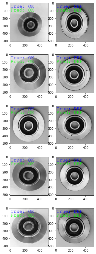
As you can see, you’ve trained a very accurate model. It is delivering around 99% on accuracy, as well as precision and recall. Let’s see how the model predicts on the sample images we explored earlier. To load models from disk, follow the instructions in the guide to inference.
[10]:
import os
import tensorflow as tf

model = tf.keras.models.load_model(f'{os.path.expanduser("~")}/model_output/session-00019/saved_model')
inference_func = model.signatures["serving_default"]

def predict(image):
    image =  tf.convert_to_tensor(image)

    logit = inference_func(image=image)['prediction']
    # BUG: Up to 0.5.2, the output of this model is a logit:
    # * Positive corresponds to any value greater than zero.
    # * Negative corresponds to any value less than zero.
    #
    # Starting in 0.5.3, the output of this model will be in the range [0, 1]:
    # * Positive generally corresponds to any value greater than 0.5.
    # * Negative generally will correspond to any value less than 0.5.
    pred = tf.nn.sigmoid(logit)
    pred = pred[0][0]
    return 'OK' if pred < 0.5 else 'DEF'

f, axarr = plt.subplots(ROWS, COLUMNS, figsize=(5,15))
curr_row = 0

for col, image_col, true in ((0, ok, 'OK'), (1, def_, 'DEF')):
    for row, image_row in enumerate(image_col):
        with PIL.Image.open(image_row) as image:
            pred = predict(image)

            drawing = PIL.ImageDraw.Draw(image)
            font = PIL.ImageFont.truetype('FreeMono.ttf', 65)
            drawing.text((10, 10), f'True: {true}', font=font, fill =(0, 0, 255))
            drawing.text((10, 60), f'Pred: {pred}', font=font, fill =(0, 255, 0))
            axarr[row, col].imshow(image)
WARNING:tensorflow:No training configuration found in save file, so the model was *not* compiled. Compile it manually.
Deployment
Now that you have a trained model, it’s time to start thinking about how you’ll integrate it with an application that your quality inspection staff will use. In your case, assume you’ve decided to hand out Apple iPhones to your quality inspectors. Look into Apple’s SDK to integrate Tensorflow Models with iOS apps to get started packaging your model into an app for your quality inspectors.